When a system of linear equations admits no exact solution, the Moore–Penrose pseudoinverse provides a canonical “best-fit” solution. In data science this is applied for the closed form solution of polynomial regression. It can be shown quite neatly how the pseudoinverse can be derived from — and is equivalent to — the problem of minimizing the least square error function over feature transformations of the model inputs. In the following, I will give a step-by-step transformation of the derivative of the general error function to the Moore–Penrose pseudoinverse.
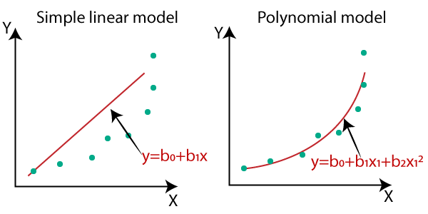
Imagine we have a dataset \(X = [x_0, …,x_n]\) and targets \(t = [t_0, …, t_n]\) where \(t_n\) is the known target value for the datapoint \(x_n\). Our goal is to fit a non-linear, polynomial curve $$y(x) = w_0 + w_1 x^1 + … + w_m x^m$$ to the target values where \(y(x_n)\) is an estimator of the target \(t_n\) and \(w = [w_0, w_1, …, w_m]\) are weight coefficients that determine the slope of the curve, and thereby the model.
To express this in the vector space we denote the \(m\)th polynomial of \(x\) as \(\phi(x) = [x, x^1, …, x^m]\) and an \(n*m\) matrix \(\Phi\) as well as \(n\)-dimensional vector \(t\) as
$$ \Phi = \begin{bmatrix} \phi(x_0)\\ \phi(x_1)\\ …\\ \phi(x_n) \end{bmatrix} $$
$$ t = \begin{bmatrix} t_0\\ t_1\\ …\\ t_n \end{bmatrix} $$
Our model can thus be specified as $$\Phi w \approx t$$
How do we find the weight vector w?
A common way to fit a regression curve is the principle of least squares: minimizing the sum of the squares of the distances between the estimator \(y(X)\) and targets \(t\). The error function to minimize over the weight matrix \(w\) can be expressed as $$ E(w) = \frac{1}{2} || \Phi w – t ||^2$$ where \(||v||\) is the length or euclidean norm of vector \(v\). The factor \(\frac{1}{2}\) is irrelevant but will tidy up the resulting closed-form solution.
To minimize the error function we expand the equation, take the gradient of \(E(w)\) and solve the resulting expression for 0. To begin, we write out the euclidean norm and expand the resulting expression. We apply some transformations relying on the properties of matrix arithmetics.
$$
E(w) = \frac{1}{2} {\sqrt{ (\Phi w – t)^T (\Phi w – t)}}^2\\
E(w) = \frac{1}{2} (\Phi w – t)^T (\Phi w – t)\\
E(w) = \frac{1}{2} ((\Phi w)^T – t^T) (\Phi w – t)\\
E(w) = \frac{1}{2} ((\Phi w)^T \Phi w – t^T \Phi w – (\Phi w)^T t + t^T t)\\
E(w) = \frac{1}{2} (w^T \Phi^T \Phi w – t^T \Phi w – (\Phi w)^T t + t^T t)\\
$$
Since \(\Phi w\) and \(t\) are both vectors multiplying them results in a scalar value. Generally, for any two vectors \(v_0, v_1\) of the same dimension and one of them transposed multiplication is commutative and \(v_0^T v_1 = v_0 v_1^T \) holds. With this we can contract the subtractive terms to get $$E(w) = \frac{1}{2} (w^T \Phi^T \Phi w – 2 t^T \Phi w + t^T t)$$
Now we take the gradient of the error function \(\frac{\partial E(w)}{\partial w}\) w.r.t. \(w\) which is a scalar by vector derivative. We can make use of matrix calculus rules. In the first term we can use the identity \(\frac{ \partial x^T A x}{ \partial x} = 2 A x\) which is a special case if \(A\) is a symmetric matrix which is the case for \(\Phi^T \Phi\) since a matrix multiplied by its transpose is always symmetric.
For the second term we apply \(\frac{\partial b^T A x}{\partial x} = A^T b\) which holds for a vector \(b\) which is not a function of \(x\). The third term vanishes. This produces: $$\frac{\partial E(w)}{\partial w} = \frac{1}{2} (2 \Phi^T \Phi w – 2 \Phi^T t)$$
Now we simplify and solve for zero.
$$\Phi^T \Phi w – \Phi^T t = 0\\
\Phi^T \Phi w = \Phi^T t\\
w = (\Phi^T \Phi)^{-1} \Phi^T t$$
Notice the last step here is achieved by left multiplying both sides with \((\Phi^T \Phi)^{-1}\).
What we end up with here is the weight vector \(w\) with the optimal coefficients for a curve fitting the target data points. The resulting expression contains the Moore-Penrose (pseudo) inverse \(A^+ = (A^T A)^{-1} A^T \approx A^{-1} \)which can be used to find the closest solution to an unsolvable system of linear equations. We remember how we expressed the model as \( \Phi w \approx t\). As this is not solvable for \(w\) by inverting \(\Phi\) which is not invertible, we can use the pseudo inverse to solve this. We have shown here that this can be directly derived from and equates to the concept of least squares error minimization.